About This Report
This report reads your land through continuous GIS data and satellite monitoring going back to 2018, currently. A large number of satellite sensor platforms (see methodology) feed through an ecoregion- and regime-aware scoring engine to produce what we call the Land Health Score.
The four ecosystem processes drive the verdict. The water cycle (how rain lands and stays); energy flow (how plants capture and store sunlight); the mineral cycle (how nutrients turn over); and community dynamics (how the plant assembly works as a functional system). Together they shape the property’s ability to absorb shocks, recover from disturbance, and build productive capital over time.
We score relative to a reference state that fits your land’s ecoregion, climate brittleness and management regime. A grassland in a non-brittle Atlantic climate is scored against grassland norms for that setting; a forest stand is scored against closed-canopy reference; agroforestry is scored against agroforestry references. The verdict you read is calibrated to your land.
The report leads with the Verdict and the Strategic Brief; read these first. Then drill into the chapters that matter to your question. Treat the numbers as indicative, not advisory: a strong direction-of-travel signal, suitable for planning, baseline-setting and disclosure, but not a substitute for ground inspection where a material decision rides on the answer.
Indicative Use Only
Thank you for being part of EcoIntel’s journey! We are building a platform to help everyone understand their land and build a healthier relationship with it. We couldn’t do it without you.
What you’re seeing is substantive and comprehensive, but it is not yet complete.
This report is indicative, not advisory. It cannot constitute formal ecological, agricultural, financial, or land management advice and should not be treated as such.
Section 1: Atlas
Each page below shows one analytical layer mapped over the property, followed by a brief explanation of what the layer represents and what to look for. Layers that aren’t available for this property (because the underlying assets weren’t generated, or because the GEE asset hasn’t been updated) are omitted automatically.
Orientation: the property in its landscape
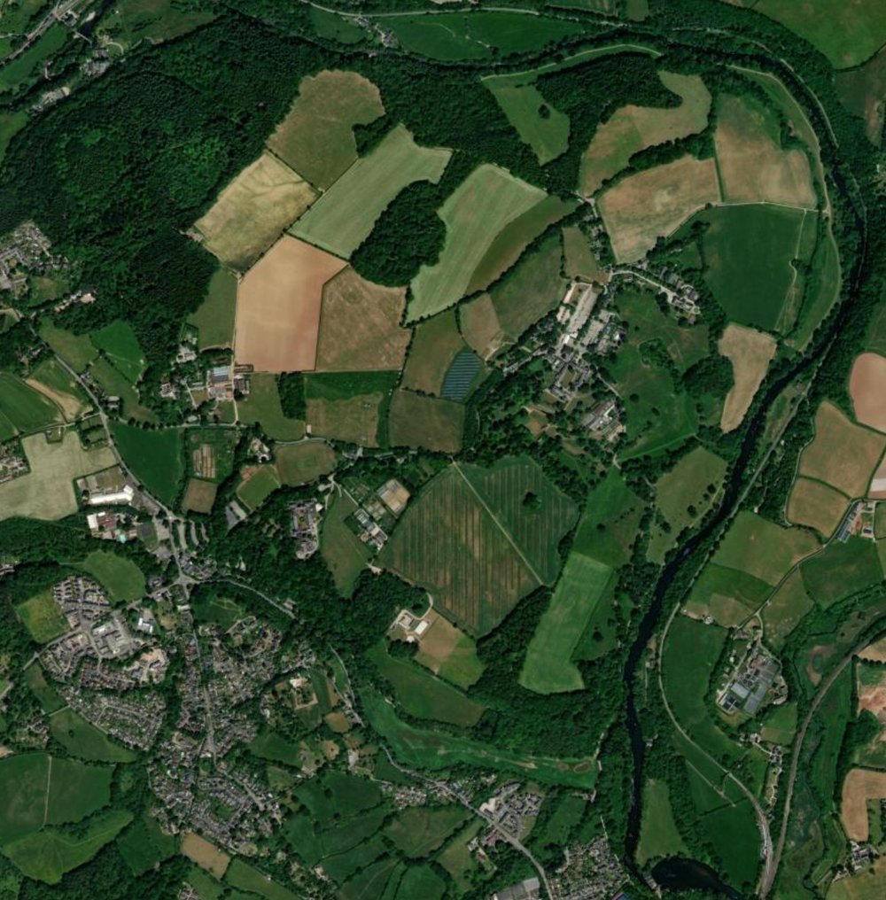
The orientation map is the starting point: the property as a satellite sees it, with no analytical overlay. The image is a high-resolution mosaic of recent cloud-free imagery so the colour and texture you see is roughly what the land has looked like in the current and previous growing seasons. Read this map first to fix your bearings: where is north, where is the property edge, what surrounds it. Pay attention to the wider landscape, the dominant land uses of the neighbours, the woodland-grassland-arable mosaic the property sits inside, the drainage lines and watercourses visible from above, the road and track network that determines access. The texture of the property’s own fields compared with the immediate neighbours is informative: if your land is the only one in the area showing dark-green continuous canopy in mid-summer, that itself is an observation. Equally if your fields show a different rotation rhythm, your fields green when the neighbours are bare, or vice-versa , the contrast points to your management decisions. This is the canvas on which every other map in the Atlas overlays its analytical layer. Most readers find it useful to come back to this image when one of the later analytical maps shows an unexpected pattern, because the unaltered satellite view often suggests an immediate physical explanation (a patch of trees, an access track, a watercourse) that the analytical layer alone cannot.
Parcels labelled
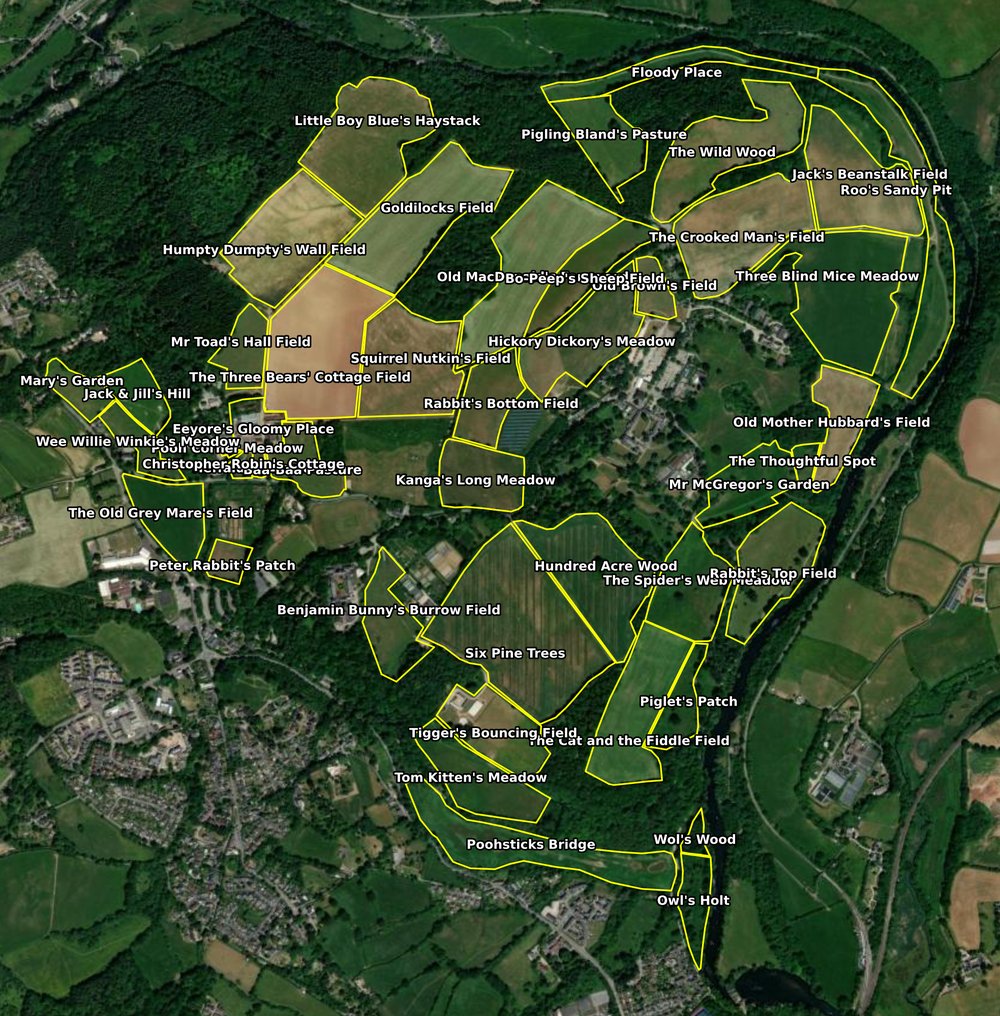
The labelled parcels map adds the property boundary and the individual parcel polygons over the satellite background, with each parcel named. Use this as the reference for everything per-parcel elsewhere in the suite: when the Land Health Report cites a specific parcel by name, when the Field Operations Profile gives operational advice for one field, when the trajectory discussion separates the recovering parcels from the declining ones, this is the map that anchors each name to a location on the ground. The polygon structure matters analytically as well as logistically. Every per-parcel score in this report is computed by aggregating satellite pixels within one of these polygons, so the polygon boundary is the resolution limit of any parcel-level statement. If two adjacent parcels are managed similarly but split for historical reasons, their scores will be close and the difference is noise. If two adjacent parcels are managed differently, a hay field next to permanent pasture, an arable rotation next to a woodland strip, the parcel boundary is doing meaningful analytical work and the scores should separate. Spotting the parcels where the boundary reflects a real management difference is one of the quickest ways to identify the next operational lever.
Topography: landform and contours
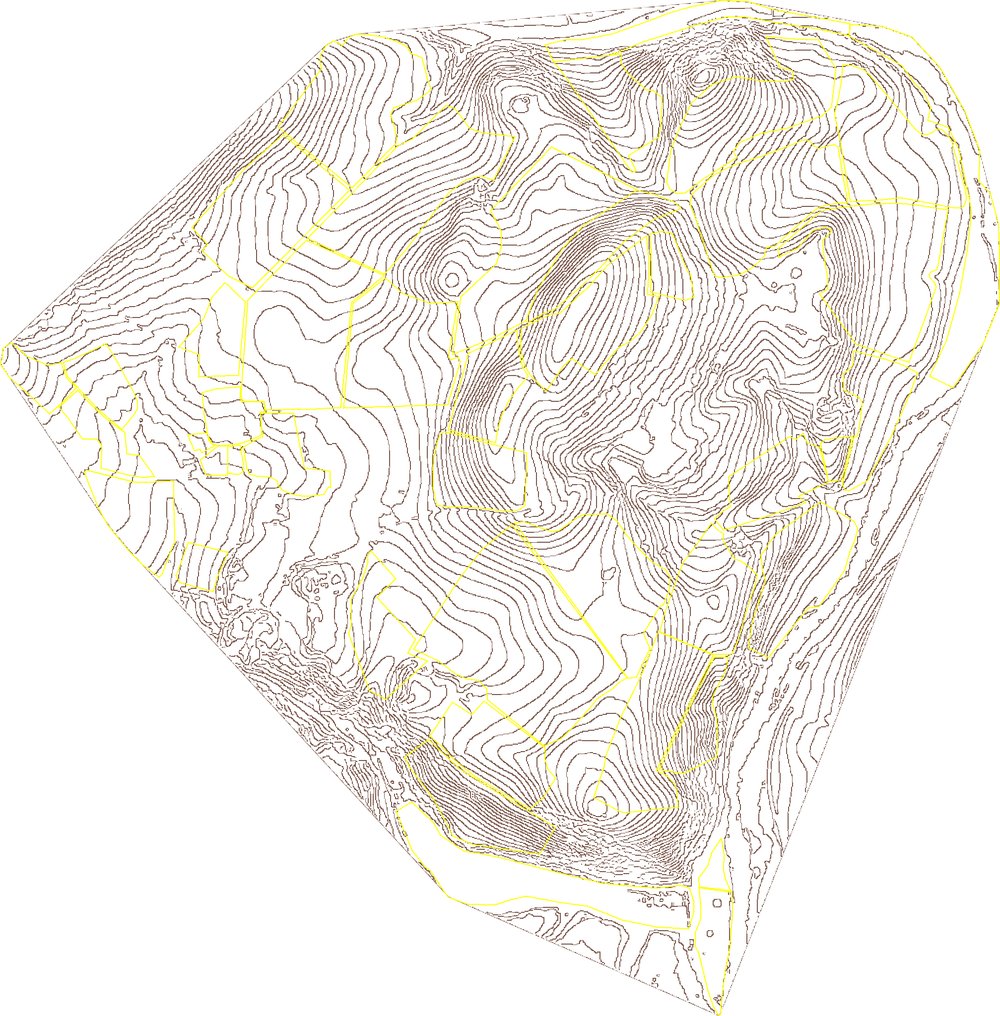
The contour map shows the shape of the land at 2 m vertical intervals. Close-spaced contours indicate steep ground; wide-spaced contours indicate flat or gently rolling terrain. The pattern of contours reveals ridges (contours curving outwards down-slope), valleys (contours curving inwards up-slope), saddles between two summits, and the natural drainage lines water follows after rain. Read the contour map alongside the orientation map: where the contours bunch, the satellite imagery often shows the change in vegetation cover that comes with steep ground, hedgerow lines along contours, bracken or scrub on the steepest faces, shorter grass on south-facing slopes. The contour reading is the foundation for the keyline-zones, ridge-network, valley-network, and topographic-wetness maps that follow. It is also the foundation for any keyline-design or contour-based intervention: tracks, swales, shelter planting, and water-harvesting features all reference these lines. For property-level planning the contours tell you three things at a glance: how much of the property is flat enough for mechanical operations, where the steep ground concentrates (and therefore where the erosion risk concentrates), and how water will move across the property in heavy rainfall.
Keyline zones
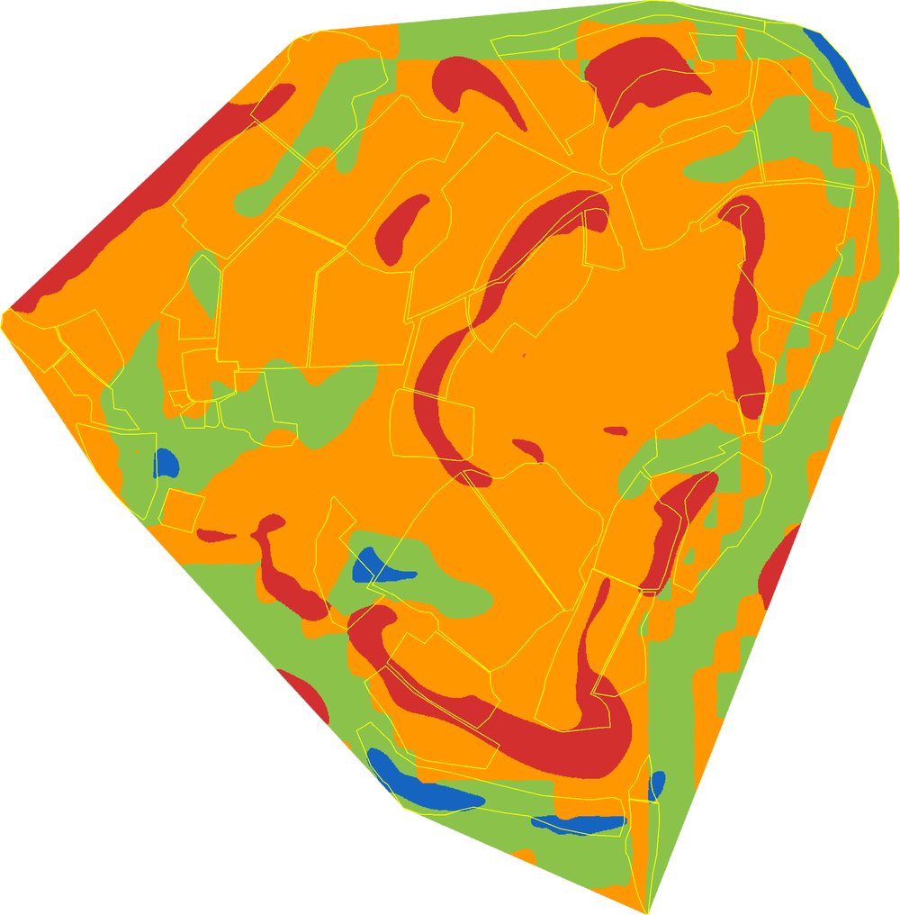
Keyline zones classify each parcel by its position in the site’s water-flow geometry, following the classical P.A. Yeomans framework. Zone 1 sits highest in the catchment, ridge tops and high shoulders that shed water in all directions. Zone 2 is the upper slope, still net-shedding but with some downslope concentration. Zone 3 is the lower slope and shoulder where water from above is starting to concentrate. Zone 4 is the valley floor and low-collecting basin where water gathers in any significant rainfall. The zone composition of the property tells you what the natural water architecture is: a property that is mostly Zone 1 and 2 needs infiltration interventions (swales on contour, key points, mulch or cover that slows surface flow); a property that is mostly Zone 3 and 4 needs storage interventions (ponds, scrapes, wet meadows) and protection against compaction in the wet months. A property that spans all four zones has the most flexibility: water can be slowed in the high zones, stored in the middle zones, and used productively in the low zones. The zone read also tells you which parts of the property are most vulnerable to drought (high zones lose water fastest) and which are most vulnerable to waterlogging (low zones receive runoff from above as well as direct rainfall).
Ridge & valley network
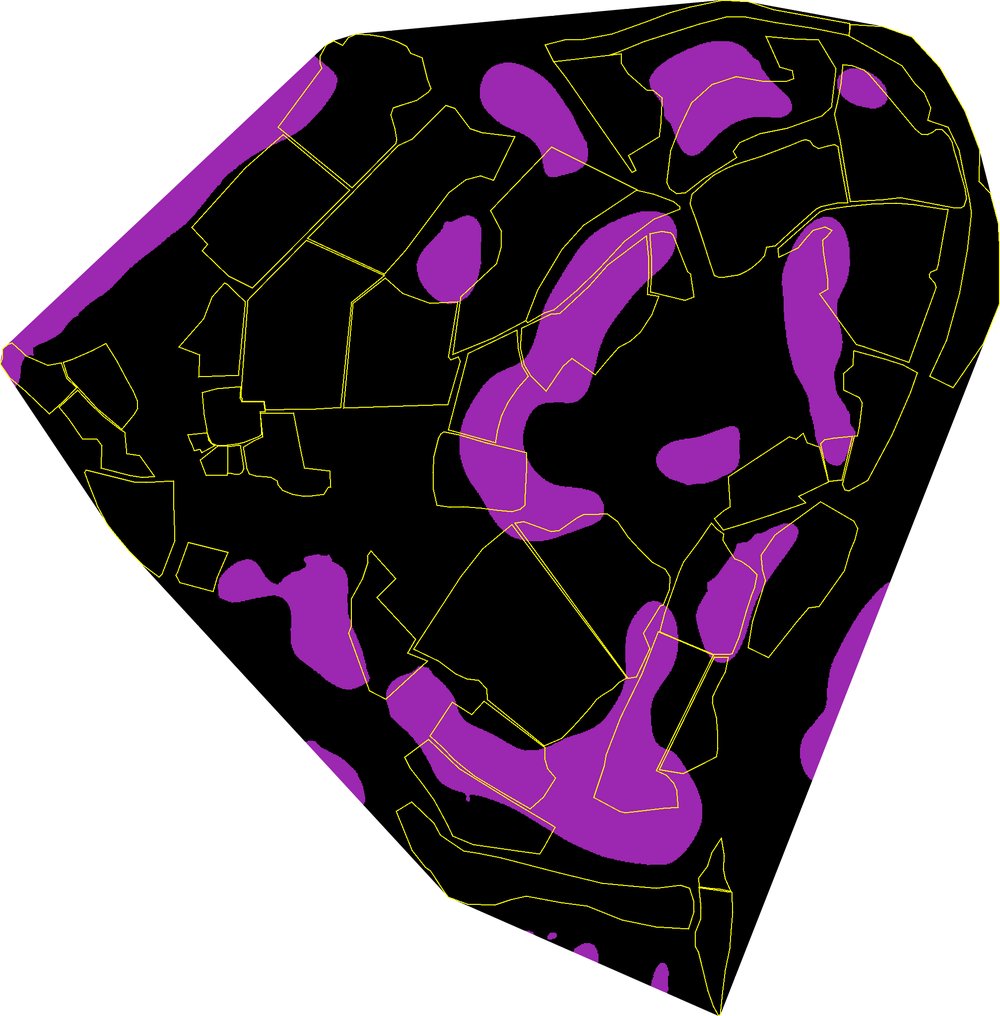
The ridge network identifies the watershed lines, where rain on one side of the line flows in one direction and rain on the other side flows in another. Ridges are where water sheds; they are typically the driest ground and historically the right place for access tracks, fence lines, hedgerows, shelterbelts, and any infiltration intervention that wants to slow water at the highest point in the catchment. Reading the ridge network alongside the parcel boundaries reveals one of the most useful operational signals on the property: parcels that sit ASTRIDE a ridge have two distinct water regimes inside a single management unit. The one side drains one way and behaves one way, the other side drains the other way and behaves differently. If a parcel is split by a ridge, the satellite scores often show internal heterogeneity that averaging across the whole parcel hides. Sub-dividing such a parcel, either operationally (two rotations, two grazing densities) or physically (internal fencing along the ridge), is sometimes the cheapest land-health intervention available, because it lets each half of the parcel be managed to its actual water regime instead of to the average. Ridges are also the natural place to plant: tree and hedge roots on a ridge stabilise the dividing line between two sub-catchments and provide shelter for both sides.
Valley network
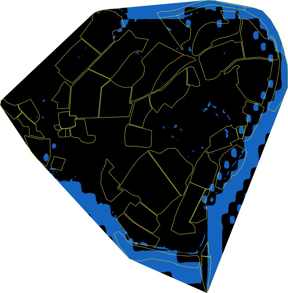
The valley network is the inverse of the ridge map: it traces where water concentrates after rain. Valleys are the wettest ground on the property, typically the most fertile (because they collect nutrient-rich runoff from upslope), and the riskiest for soil loss during heavy events (because the same concentrated flow that delivers nutrients can also carry soil downstream). Valley-bottom parcels typically have higher baseline productivity but also higher vulnerability to compaction (the wet ground is soft, so machinery and stock leave a deeper print) and to nutrient export (water leaving the property carries with it whatever the soil cannot hold). Cross-reference with the keyline-zones map: valleys map onto Zone 3 and Zone 4 positions. Cross-reference with the topographic-wetness map: the valley network is the geometric skeleton; the wetness index is the analytical surface over that skeleton. Operationally, the valley network shows where to place water-storage interventions (ponds, scrapes, wet meadow extensions), where to set back arable rotations to reduce nutrient loss, and where riparian buffers, even narrow ones, earn the most ecological return.
Topographic wetness (TWI)
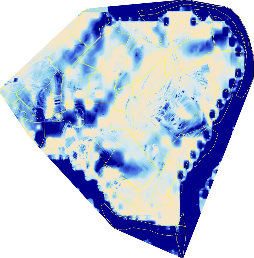
The Topographic Wetness Index (TWI) combines slope and upslope catchment area into a single index of where water concentrates. The calculation is based on the LIDAR DTM and is independent of weather: it reflects the permanent geometry of the land, not the rainfall pattern of any given year. High TWI areas (the brighter blues on the map) have large catchments draining into a shallow slope, these are the places that stay wet longest after rain and are most likely to flood in heavy events. Low TWI areas (the darker tones) have small catchments or steep slopes, these drain freely and dry quickly. The TWI surface is the satellite-derived proxy for the wet-ground / dry-ground distinction that any experienced observer would notice walking the property in late winter, but the satellite version is consistent across the whole property at the same resolution. Read TWI alongside the EDX-by-year map: where high TWI coincides with declining EDX, the parcel may be getting wetter than the management is accounting for (rising water table, blocked drainage, recent loss of upslope cover). Where low TWI coincides with declining EDX, the parcel may be getting drier than historically, early-season drought signal.
Landform position
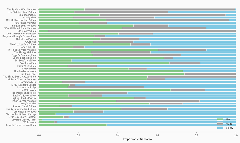
Landform position classifies each pixel as ridge, slope, valley, or flat, a four-class summary of where on the topographic gradient the pixel sits. It is the most direct topographic-context map: at a glance you see which parts of the property sit in each landform class, and what the proportions are overall. A property that is 80 % slope and 20 % flat behaves very differently from one that is 80 % flat and 20 % slope, even if both have the same total area and the same headline scores. The landform classification is also a useful sanity check on the ecosystem-process scores: ridge parcels should show drought signal earlier than flat parcels in the same property; valley parcels should show waterlogging signal earlier than ridge parcels in the same property; flat parcels should be the most management-sensitive (because they are not weather-bound to landform). When the ecosystem-process scores don’t follow this expected gradient, a valley parcel that scores lower than a ridge parcel in the same property, for example, there is usually a management explanation that the analyst should explore. Combined with the keyline-zones map this layer gives the most efficient summary of the property’s physical character.
Land Health (EDX), latest year
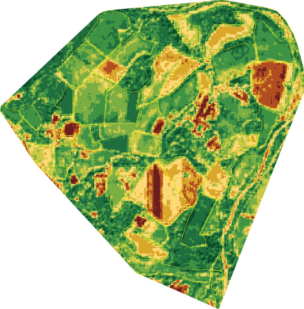
The EDX map shows the Land Health Score band per parcel in the most recent assessment year. The colour ramp runs from deep red (EDX1 Collapsed, below ~31 % of potential) through gold (EDX4-5 Stressed / Transitional, ~46-62 %) to deep green (EDX8-9 Thriving / Flourishing, ~77-100 %). This is the single most-referenced map in the report suite: it answers the headline question “where is the land healthy today, and where is it not?” at the same parcel resolution the rest of the analytical pipeline sees the property. Read it three ways. First, the property average: what band is the property settling into overall? Second, the spread: are all parcels in the same band (uniform management, uniform conditions) or do they span several bands (heterogeneous management, or heterogeneous landform driving different baselines)? Third, the outliers: individual parcels two or more bands above or below the property average. The high outliers are the demonstration parcels, what the rest of the property could look like with the right combination of management and time. The low outliers are the first-call diagnostic priority, the parcels where something specific is happening that the rest of the property is not exposed to.
Land Health trajectory
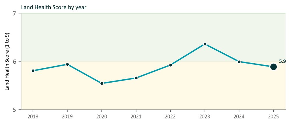
The trajectory line shows the property’s site-aggregated Land Health Score across the assessment window. Look for three things, in order. First, the BAND: which EDX band has the property been settling into? A property that is consistently in EDX5-6 is in a different position from one that is consistently in EDX7-8, even if the year-to-year shape is the same. Second, the SLOPE: rising, falling, or steady? A rising slope is the strongest evidence that management is delivering. A falling slope is a signal to investigate, though a single dry year can pull a slope down without the underlying condition having changed. A steady slope in a high band is stable productivity; a steady slope in a low band is locked-in degradation. Third, the DIPS and SPIKES: single-year departures from the local trend. A weather-driven dip is usually one year wide, recovers immediately, and coincides with a recorded dry or wet event. A management-driven dip persists for more than one year and corresponds to a specific change (rotation shift, stocking change, contractor change, land-use change). The trajectory verdict in the Strategic Action Brief is derived from this multi-year shape; this map is the visual source for that verdict.
Carbon balance: site flux
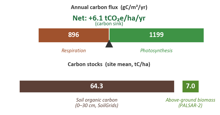
The site carbon-balance figure shows photosynthesis (GPP, the carbon coming in via plant growth) against ecosystem respiration (Reco, the carbon going out via plant and soil-microbe respiration) and net biome production (NBP, what is left over after both flows and any export of biomass). The beam-and-fulcrum visual makes the headline question, is this land building carbon or losing it?, immediate. NBP greater than zero means the property is a net carbon sink across the assessment window: more carbon is being fixed into soil and biomass each year than is being lost back to the atmosphere or exported. NBP less than zero means the property is a net carbon source: the land is releasing more carbon than it is fixing. The size of the imbalance matters as much as its sign. A small positive NBP indicates near-neutral land that could tip either way under a different management regime; a large positive NBP indicates land that is actively building carbon at a rate comparable to the best regenerative case studies. The figure is calibrated to MODIS GPP at the site level so the absolute numbers are tied to satellite consensus; per-parcel partitioning is less reliable than the site total. Read this figure with the cumulative-sequestration chart on the next page.
Cumulative carbon sequestration
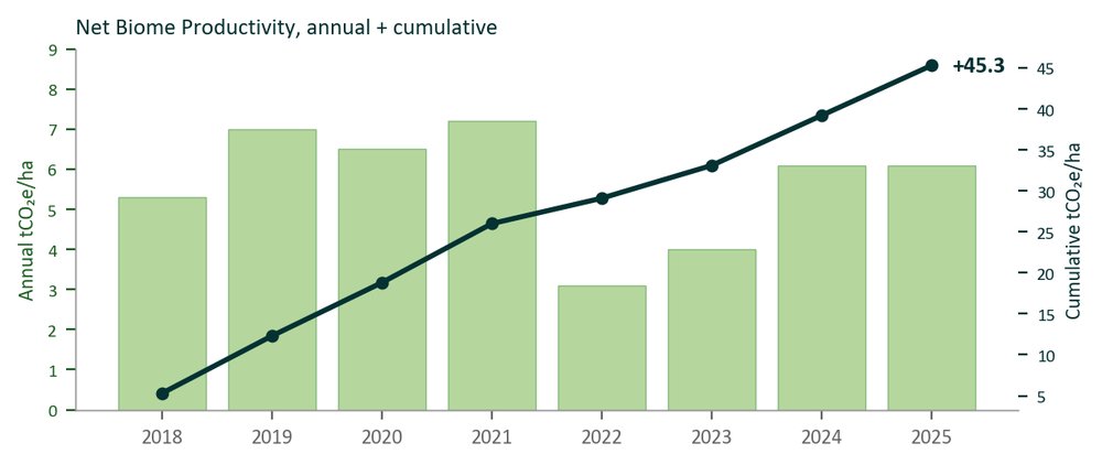
The cumulative chart adds NBP year-by-year into a running total of carbon stocked or lost across the assessment window. A rising line means the property has been building soil-plus-biomass carbon throughout, the trajectory is positive and the magnitude of the gain is the height of the line. A flat line means net-neutral: gains in some years cancel losses in others. A falling line means net carbon loss. The slope of the line is the rate of carbon accumulation per year averaged across the property; a steeper slope means a faster rate. Read the cumulative chart with the site carbon-balance figure on the previous page: the balance shows the average annual flux, the cumulative chart shows what that flux integrates to. A property with a small positive average flux and a long assessment window can still accumulate meaningful carbon; a property with a large positive flux but a short window is signalling potential but has yet to demonstrate it. Where the cumulative line bends mid-window, look back at the trajectory line: major changes in EDX often correspond to changes in the carbon-accumulation rate as the underlying process scores shift.
Disturbance timeline
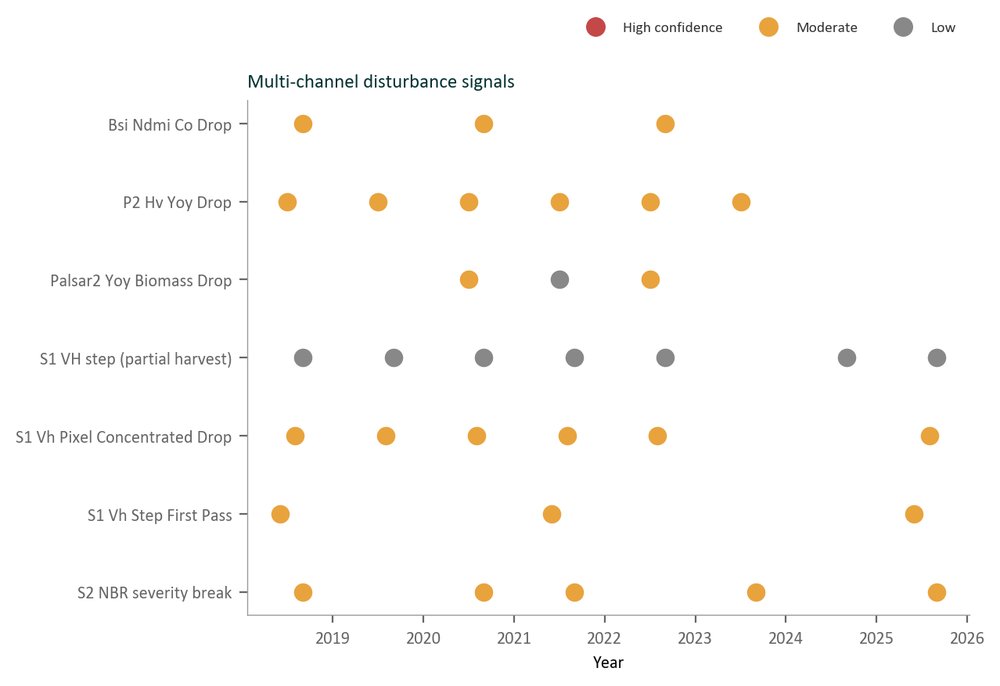
The disturbance timeline marks individual events the satellite stack detected over the assessment window, sudden drops in green vegetation, canopy loss in forest parcels, exposure of bare soil after ploughing or heavy poaching, fire scars, harvested-field signals. Each marker corresponds to a specific date (the satellite revisit week in which the change was first detectable) and a specific parcel (the polygon inside which the disturbance occurred). Where multiple parcels show the same disturbance week, the cause is usually weather (storm, drought break, frost event) or systemic (a rotation step across many fields, a contractor working the whole property in one pass). Where a single parcel shows a disturbance the rest of the property did not, the cause is usually parcel-specific (a localised cut, a herd movement, a tree-fall, a contractor intervention). The timeline is the audit trail for any investigation into a single year’s scores: a parcel that drops a band in one year usually has a corresponding disturbance entry that explains why, and the entry pins the explanation to a specific week rather than the whole year.
Opportunities map
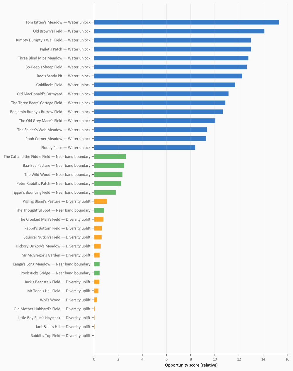
The opportunities map highlights where the satellite analysis has identified specific potential interventions on the property, infiltration features in high-keyline-zone parcels, pond and scrape suitability in low-keyline-zone parcels, hedge or shelterbelt opportunities along exposed boundaries, recovery targets in below-average-performing parcels, shade-tree opportunities for stock fields lacking summer cover. Each highlight is anchored to a specific parcel and a specific opportunity class so the strategic conversation about “how do we develop this property?” can move from the abstract to the concrete. Read the opportunities map alongside the Strategic Action Brief’s Opportunities section for the underlying logic behind each highlight: each opportunity on the map has a corresponding paragraph in the brief explaining the ecological reasoning, the typical capital and time commitment, and the most-likely outcome pathway. The map is not a prescription, it is a starting set of analytically-grounded candidates that the property manager and any design partner can rank, refine, and combine into an actual programme of work.
Risk matrix
The risk matrix plots property-level risks across three axes: ecological (vulnerability to ecosystem-function loss), financial (productivity decline that translates into income decline), and compliance (readiness to evidence the disclosure frameworks this report supports, including TNFD, ESRS E4, GRI 101, SBTN and EUDR). Cells in the top-right are higher-priority risk areas; cells in the bottom-left are lower-priority. The matrix is the strategic counterpart to the opportunities map: opportunities answer “what could go better?”, risks answer “what could go wrong?” The two together form the full strategic picture of the property. Read each risk with three questions in mind. First, what is the trigger event, the specific thing that would have to happen for the risk to materialise (a multi-year drought, a regulatory change, a key-supplier failure)? Second, what is the lead indicator, the thing the satellite or operational data would show before the trigger event arrived (a multi-year decline in WCI for drought risk, a divergence between GPP and Reco for soil-carbon risk)? Third, what is the mitigation, the design or management change that would shift the risk from top-right to bottom-left over the next three to five years?

Section 2: Methodology & Confidence
Data Sources
Source | Res. | Revisit | Role |
|---|---|---|---|
Sentinel-2 MSI | 10 m | 5 day | Optical: 12 spectral indices |
Sentinel-1 C-SAR | 10 m | 12 day | Radar: VH, VV |
PALSAR-2 L-SAR | 25 m | Annual | Radar: HV (woody biomass) |
Landsat 8/9 TIRS | 100 m | 16 day | Thermal: LST, cooling |
ECOSTRESS | 70 m | Variable | Thermal: ISS orbit |
MODIS MOD17A2H | 500 m | 8 day | GPP calibration |
GEDI L4A | 25 m | Sparse | Lidar: AGB |
SMAP L4 | 9 km | Daily | Soil moisture |
Dynamic World | 10 m | Per-scene | Land cover (9 classes) |
ERA5-Land | 11 km | Daily | Climate variables |
SoilGrids | 250 m | Static | SOC, clay, nitrogen |
UK LIDAR | 1-2 m | Static | High-res DEM |
Scoring Framework
Land Health Scoring Framework
EcoIntel scores four ecosystem processes (Energy Flow, Water Cycling, Mineral Cycling, Community Dynamics) using weighted composites of optical indices, radar structure, and soil/litter proxies. Process scores (0-100%) are converted to a 9-level EDX classification. An 8-model weather-corrected ensemble using spectral, temporal, radar, topographic, and climate predictors. Models G and H incorporate growing-season stress weeks and evapotranspiration ratio to separate weather effects from ecosystem health. Cross-validated performance: R²=0.55, MAE=11 points, r=0.79.
Confidence Assessment
Confidence reflects the length of the assessment record and the availability of calibration data. Longer records (5+ years) provide HIGH confidence because they capture inter-annual variability and reveal genuine trends rather than single-year snapshots.
Assessment period: 8 years (2018-2025). Confidence: HIGH.
What Remote Sensing Can and Cannot Detect
Can Detect | Cannot Detect |
|---|---|
Vegetation vigour, cover, seasonal dynamics (10 m) | Individual plant species |
Canopy structure and woody biomass (25 m) | Soil biology (fungi:bacteria, earthworms) |
Soil moisture trends (10 m radar) | Root depth and architecture |
Land surface temperature (70-100 m) | Soil aggregate stability |
Multi-year productivity trends | Management intent |
Carbon flux estimation | Soil chemistry (pH, nutrients) |
Ecological Knowledge Base
The diagnostic interpretations in this report draw on a curated knowledge library of ecological principles. These include:
- Aspect-based seasonal management, how solar angle, slope, and aspect influence grazing timing, recovery periods, and drought vulnerability across the landscape.
- Brittleness ecology, the relationship between rainfall variability and ecosystem management requirements, following the Savory brittleness continuum.
- Diagnostic matrix framework, structured gap-pattern analysis linking process scores to root causes and management prescriptions by farming system.
- Keyline design principles. Yeomans-based water harvesting geometry for landscape water management.
- Soil management, soil health indicators, compaction dynamics, and organic carbon management principles.
- Vegetation indicator ecology, ecological interpretation of spectral indices and their relationship to ecosystem processes.
- Regional geology and soils, soil type characteristics and their implications for land management.
These principles are applied programmatically through the diagnostic matrix and inform the site-specific interpretations throughout this report. The knowledge base is maintained by Ecological Intelligence and draws on published ecological science.
Glossary
Water Cycle Index (WCI)
| Level | Range | What this level means |
|---|---|---|
| 9Flourishing | 95-100% | The landscape acts as a sponge, rainfall infiltrates fully and soils hold steady through extreme events. |
| 8Thriving | 90-95% | Excellent infiltration with rare runoff. The water cycle is doing its job through normal storms. |
| 7Healthy | 85-90% | Good infiltration with only occasional runoff in heavy rain. Soils are mostly stable. |
| 6Recovering | 80-85% | The water cycle is working but with some runoff during storms. Foundations are sound and the room to improve is in capture and retention. |
| 5Transitional | 70-80% | A transitional water cycle, working in places, weakening in others. Targeted landscape design (keyline, swales, ponds) would unlock real gains. |
| 4Stressed | 60-70% | The water cycle is weakening across the system, frequent sheet flow and pedestals around plants signal active soil loss. |
| 3Degraded | 50-60% | Significant dysfunction in the water cycle, rills and runoff are common across the landscape. |
| 2Depleted | 40-50% | Severe weakening of the water cycle; most rainfall is lost to runoff and the soil surface is widely capped. |
| 1Collapsed | 0-40% | The water cycle has effectively collapsed, rainfall runs off immediately and erosion is severe. |
Energy Flow Index (EFI)
| Level | Range | What this level means |
|---|---|---|
| 9Flourishing | 95-100% | Peak photosynthetic capacity throughout the year, the system captures all available solar energy. |
| 8Thriving | 85-95% | Strong biomass production with a stable canopy through normal disturbance. |
| 7Healthy | 75-85% | Healthy canopy growth with only brief stress-related dips. |
| 6Recovering | 60-75% | The canopy is doing real work, with seasonal stress dips that recovery has not yet smoothed out. Energy capture is on the right side of the curve. |
| 5Transitional | 40-60% | Energy capture is uneven across the year, strong in spring, weakening in summer. Recovery management would lift this further. |
| 4Stressed | 30-40% | A thin canopy with patchy litter; the system is producing biomass but slowly and unreliably. |
| 3Degraded | 20-30% | Low photosynthetic capacity even in growing season; canopy is sparse and slow to respond. |
| 2Depleted | 10-20% | Very low photosynthesis; the canopy is nearly absent for much of the year. |
| 1Collapsed | 0-10% | Canopy has collapsed or is dominated by standing dead material. |
Mineral Cycle Index (MCI)
| Level | Range | What this level means |
|---|---|---|
| 9Flourishing | 90-100% | Rapid, complete nutrient cycling, the soil builds organic matter continuously. |
| 8Thriving | 80-90% | Strong mineral cycling with fast litter incorporation and high microbial activity. |
| 7Healthy | 70-80% | Good mineral turnover with only occasional seasonal slow-down. |
| 6Recovering | 60-70% | Mineral cycling is working but slows in dry or cold periods. The biological engine is in place, the next step is to keep it warm year-round. |
| 5Transitional | 50-60% | Litter is starting to accumulate without breaking down; cycling is uneven across the site. |
| 4Stressed | 40-50% | Poor litter incorporation, nutrients are locked in undecomposed material on the surface. |
| 3Degraded | 30-40% | Mineral cycle largely broken; bare ground and compacted surfaces are common. |
| 2Depleted | 20-30% | Active erosion is stripping soil and nutrients; cycling has effectively collapsed. |
| 1Collapsed | 0-20% | Soil mineral cycle is non-functional and nutrient cycling has effectively collapsed. |
Community Dynamics Index (CDI)
| Level | Range | What this level means |
|---|---|---|
| 9Flourishing | 85-100% | Rich functional diversity across all groups; rare species thrive. |
| 8Thriving | 75-85% | Well-structured communities with low presence of undesirable species. |
| 7Healthy | 65-75% | Healthy functional groups; rare species appear occasionally. |
| 6Recovering | 55-65% | Diversity is recovering, the foundation species are in place and the rarer functional groups are working their way back in. |
| 5Transitional | 45-55% | Some functional groups are uneven, and undesirable species are starting to gain ground. Extended recovery periods are the lever here. |
| 4Stressed | 35-45% | Key functional groups are noticeably weakening; diversity is declining. |
| 3Degraded | 25-35% | Undesirable species are common; rare species rarely seen. |
| 2Depleted | 15-25% | Functional groups are actively failing and diversity is sharply reduced. |
| 1Collapsed | 0-15% | The community has collapsed to a handful of stress-tolerant species. |
- Land Health Score
- The headline metric, a property's overall ecological condition, given as a level from 1 (Collapsed) to 9 (Flourishing) with its band label.
- Band
- The name attached to each level: Collapsed, Depleted, Degraded, Stressed, Transitional, Recovering, Healthy, Thriving, Flourishing. Each band has one fixed colour.
- EDX, Ecological Diagnostic Index
- The underlying 0-100% index from which the Land Health Score level is derived. Used in methodology only.
- EHI, Ecological Health Index
- The composite that combines the four ecosystem-process scores into the EDX value.
- Ecosystem processes
- The four functional lenses assessed on the same nine-level scale: Water Cycle, Energy Flow, Mineral Cycle and Community Dynamics.
- Evidenced · Positioned · Baseline · Documented
- Confidence language for each finding, from multiple corroborating signals (Evidenced) through to recorded but not yet corroborated (Documented). This report never uses pass / fail.
- VVB, Validation & Verification Body
- An accredited third party that verifies carbon or biodiversity claims for market use.
EDX Land Health Score
The Land Health Score classifies each property into one of nine bands. EDX is the technical name for the band number, so “EDX8 Thriving” is the same as “Land Health Score Level 8”. The entries below describe each band in detail: the ecological characteristics that define it, the typical process score ranges, and the practical steps required to move up to the next band. For an at-a-glance comparison across all nine bands see Section 1.4.1 of the Master Report; for this site’s current band see Section 2.2 of the Master Report.
See the concept introduction in Section 1.4.1 of the Master Report and Section 2.2 of the Master Report for the site-specific reading.
EDX9, Flourishing
Ecosystems not only resilient but actively improved by disturbance, with highly efficient water infiltration, negligible erosion, vigorous canopy with strong solar energy capture, and diverse communities where rare species thrive. Water cycles effectively with minimal runoff, soils remain stable under stress, and functional groups are vigorous across the full diversity spectrum. This represents the pinnacle of ecological health where the system builds capacity through interaction with its environment.
Process | Range | Characteristics |
|---|---|---|
Water Cycling (WCI) | 95-100% | Infiltration efficient; minimal runoff |
Energy Flow (EFI) | 95-100% | High live canopy; strong capture/conversion |
Mineral Cycling (MCI) | 90-100% | Soil surface stable; negligible erosion |
Community Dynamics (CDI) | 85-100% | Diverse; desirable FGs vigorous; rares present |
Path to improvement: EDX9 represents optimal function. Maintain through adaptive management that responds to system feedback, protect rare species habitat, continue monitoring for early warning signals, and share knowledge with broader community to support regional ecosystem health.
EDX8, Thriving
Ecosystem processes are efficient and mutually reinforcing, creating robust ecological health that recovers quickly from disturbance. Good water infiltration with rare erosion events, stable soils showing no active degradation, high photosynthetic biomass production, and well-structured communities with low undesirable species presence. Systems at this level maintain function through normal climate variability and disturbance events.
Process | Range | Characteristics |
|---|---|---|
Water Cycling (WCI) | 90-95% | Good infiltration; rare rills |
Energy Flow (EFI) | 85-95% | High photosynthetic mass |
Mineral Cycling (MCI) | 80-90% | Stable; no active pedestals |
Community Dynamics (CDI) | 75-85% | Good structure; low undesirables |
Path to improvement: To reach EDX9: Enhance habitat complexity for rare species, eliminate remaining stress points in seasonal dips, fine-tune intervention timing to phenological and moisture cycles, increase functional group diversity in weak areas, and build deeper soil organic matter reserves through strategic carbon inputs.
EDX7, Healthy
Good infiltration, stable soils, strong canopy growth, and healthy community dynamics characterize this band, representing solid ecosystem function suitable for sustained productivity. Water cycles are mostly effective with occasional limitations, soils are predominantly stable, photosynthesis is robust with only short stress-related dips, and functional groups are healthy with rare species appearing occasionally. This is the threshold where regenerative management typically aims to maintain or exceed.
Process | Range | Characteristics |
|---|---|---|
Water Cycling (WCI) | 85-90% | Mostly effective; occasional limits |
Energy Flow (EFI) | 75-85% | Robust growth; short stress dips |
Mineral Cycling (MCI) | 70-80% | Mostly stable |
Community Dynamics (CDI) | 65-75% | FGs healthy; rares occasional |
Path to improvement: To reach EDX8: Address seasonal stress periods with better recovery management, increase litter cover uniformity across landscape, strengthen water infiltration in limited areas, boost functional diversity in weaker zones, and refine disturbance timing to match plant vigor cycles for faster recovery.
EDX6, Recovering
Ecosystem cycles are mostly working but with limited resilience and patchy diversity, indicating improvement from lower states but not yet fully functional. Some runoff events occur during heavy rainfall, minor soil instability is beginning to show, canopy exhibits evident seasonal stress dips, and some functional groups show weakness or patchiness. Land in this band is on a positive trajectory but requires continued management attention.
Process | Range | Characteristics |
|---|---|---|
Water Cycling (WCI) | 80-85% | Some runoff events |
Energy Flow (EFI) | 60-75% | Seasonal dips evident |
Mineral Cycling (MCI) | 60-70% | Minor instability showing |
Community Dynamics (CDI) | 55-65% | Some FG weakness/patchiness |
Path to improvement: To reach EDX7: Reduce bare ground exposure through improved canopy cover and understorey density, extend non-intervention periods between operations, address weak functional groups through enrichment planting or habitat creation, improve water distribution to eliminate dry spots, and build soil organic matter through increased litter retention and reduced soil disturbance.
EDX5, Transitional
Some ecosystem processes are holding while others are weakening, creating uneven canopy cover and diversity across the landscape. Runoff is frequent during storms, localized erosion and soil capping appear in vulnerable areas, canopy is uneven with variable vigor, and undesirable species are beginning to increase. This band represents a critical threshold where management decisions will determine whether the system improves toward EDX6 or weakens toward EDX4.
Process | Range | Characteristics |
|---|---|---|
Water Cycling (WCI) | 70-80% | Runoff frequent storms |
Energy Flow (EFI) | 40-60% | Uneven canopy |
Mineral Cycling (MCI) | 50-60% | Localized erosion/capping |
Community Dynamics (CDI) | 45-55% | Undesirables creeping |
Path to improvement: To reach EDX6: Urgent need to stop degradation trend. Immediately reduce soil disturbance, dramatically increase ground cover through enrichment planting and assisted natural regeneration, address erosion hotspots with targeted interventions, extend non-intervention periods significantly, and reduce harvesting pressure to allow ecosystem recovery. This is the last easy intervention point before major restoration becomes necessary.
EDX4, Stressed
Patchy vegetation cover, stuttering ecosystem cycles, and weakening functional group integrity characterize this vulnerable state. Water infiltration is poor with frequent sheet flow across the surface, pedestals begin to appear around plant bases indicating active soil loss, canopy is thin with patchy litter distribution, and key functional groups are noticeably weakening. Systems in this band are highly vulnerable to further degradation without significant management intervention.
Process | Range | Characteristics |
|---|---|---|
Water Cycling (WCI) | 60-70% | Poor soak; frequent sheet flow |
Energy Flow (EFI) | 30-40% | Canopy thin; litter patchy |
Mineral Cycling (MCI) | 40-50% | Pedestals appear |
Community Dynamics (CDI) | 35-45% | Key FGs weakening |
Path to improvement: To reach EDX5: Major management redesign required. Cease all extractive operations and implement canopy retention, establish emergency ground cover through pioneer nurse species, address all visible erosion with mechanical and biological fixes, implement non-intervention zones for worst areas, introduce missing functional groups through assisted natural regeneration, and develop long-term soil rebuilding strategy. Expect 3-5 year recovery timeline with intensive inputs.
EDX3, Degraded
Poor water infiltration, visible erosion signals, low photosynthetic capacity, and rising dominance of undesirable species indicate significant ecosystem dysfunction. Regular runoff and rill formation occur, erosion indicators are common across the landscape, biomass production is low with slow recovery from disturbance, and undesirable species are becoming common while rare species are rarely seen. Land in this band requires comprehensive management redesign to prevent further decline.
Process | Range | Characteristics |
|---|---|---|
Water Cycling (WCI) | 50-60% | Regular runoff; rills |
Energy Flow (EFI) | 20-30% | Low biomass; slow recovery |
Mineral Cycling (MCI) | 30-40% | Erosion signals common |
Community Dynamics (CDI) | 25-35% | Undesirables common; rares rare |
Path to improvement: To reach EDX4: Comprehensive restoration program essential. Halt all extraction immediately, implement mechanical erosion control structures, establish pioneer nurse species for canopy rebuilding and soil stabilisation urgently, protect remaining seed trees as mycorrhizal refugia, consider importing topsoil for worst areas, develop 5-10 year restoration plan with staged interventions, seek expert guidance and potentially external funding. Economic returns unlikely for many years - focus must be on stopping collapse.
EDX2, Depleted
Severe weakening of water and mineral cycles, weak canopy, and failing diversity indicate land on the edge of collapse requiring urgent intervention. Little water infiltrates with most rainfall lost to runoff, active erosion with widespread soil surface capping, low photosynthetic activity producing minimal biomass, and functional groups actively failing with sharply reduced diversity. Without immediate management changes, systems in this band are likely to collapse to EDX1.
Process | Range | Characteristics |
|---|---|---|
Water Cycling (WCI) | 40-50% | Little infiltration |
Energy Flow (EFI) | 10-20% | Low photosynthesis |
Mineral Cycling (MCI) | 20-30% | Active erosion; capping widespread |
Community Dynamics (CDI) | 15-25% | FGs failing; low diversity |
Path to improvement: To reach EDX3: Emergency restoration required. Total cessation of all disturbance mandatory, intensive mechanical stabilisation of erosion features, emergency planting of nurse species and pioneer trees with mycorrhizal inoculation where networks have been destroyed, potential need for irrigation support in establishment phase, soil amendment programs to restart biological activity, professional restoration expertise essential. Timeline 10+ years, significant investment required. Consider whether restoration is economically viable or if alternative land use needed.
EDX1, Collapsed
Water runs off immediately, severe soil erosion is active, canopy is nearly absent or dominated by standing dead material, and ecological communities have collapsed toward a handful of stress-tolerant species. Flashy water loss occurs with every rainfall event, erosion is severe and ongoing, bare ground or dead vegetation dominate the landscape, and biological diversity has effectively collapsed. This represents complete ecosystem dysfunction requiring intensive, long-term restoration intervention.
Process | Range | Characteristics |
|---|---|---|
Water Cycling (WCI) | 0-40% | Flashy water loss |
Energy Flow (EFI) | 0-10% | Bare/standing dead dominate |
Mineral Cycling (MCI) | 0-20% | Severe erosion |
Community Dynamics (CDI) | 0-15% | Collapse towards few stress-tolerant species |
Path to improvement: To reach EDX2: Requires intensive, long-term restoration commitment. Engineering solutions essential for hydrological stabilisation - terracing, check dams, retention structures. Imported soil substrate and mycorrhizal inoculum likely necessary. Phased assisted regeneration with pioneer nurse species and intensive irrigation for establishment. May require 15-20+ years and investment exceeding land value. Alternative consideration: managed retreat to less intensive land use, conservation easement, or habitat restoration with public funding support. Traditional productivity may not be recoverable.
Other Terms
Term | Definition |
AGB | Above-Ground Biomass, standing plant biomass above the soil surface, estimated from PALSAR-2 L-band radar (tC/ha) |
BNG | Biodiversity Net Gain. UK planning requirement for measurable habitat improvement |
BSI | Bare Soil Index, spectral measure of exposed soil |
Catena | Soil sequence from ridge to valley |
CDI | Community Dynamics Index, structural diversity and vegetation complexity |
CIred | Chlorophyll Index Red-edge, canopy chlorophyll concentration derived from Sentinel-2 red-edge bands |
CV | Coefficient of Variation, standard deviation divided by mean, a measure of relative variability |
DEM | Digital Elevation Model, gridded terrain height data (UK LIDAR 2m used in this report) |
Dynamic World | Google Dynamic World, near-real-time 10m land cover classification from Sentinel-2 |
ECOSTRESS | ECOsystem Spaceborne Thermal Radiometer on the International Space Station, high-resolution thermal imaging |
EDX | EcoDynamic Index, 9-level classification derived from EHI |
EFI | Energy Flow Index, photosynthetic capacity and biomass production |
EHI | Ecosystem Health Index, composite score across all four processes (0-100% scale) |
EHI~ | EHI on the ground-truth scale (−140 to +120), the closest approximation to verified ecosystem health |
EOV | Ecological Outcome Verification. Savory Institute field assessment protocol for measuring ecological health outcomes |
ERA5 | ECMWF Reanalysis v5, global climate dataset |
ESRS | European Sustainability Reporting Standards. EU mandatory disclosure framework (E1 = climate, E4 = biodiversity) |
ET/PET | Actual/Potential Evapotranspiration ratio |
EVI | Enhanced Vegetation Index, improved greenness measure that reduces atmospheric and soil background effects |
GHG Protocol | Greenhouse Gas Protocol, international corporate standard for greenhouse gas accounting |
GPP | Gross Primary Productivity, total photosynthetic carbon capture (gC/m²/yr) |
GS | Growing Season, the period of active vegetation growth, typically April-October in UK temperate climates |
GT / GT* | GT = Ground Truth (in-field ecological assessment score). GT* = weather-corrected ground truth, removing assessor bias caused by weather conditions on the day of assessment |
HV / VH / VV | Radar polarisation modes. VH = vertical-horizontal (Sentinel-1, biomass proxy). HV = horizontal-vertical (PALSAR-2, woody biomass). VV = vertical-vertical (Sentinel-1, moisture/roughness) |
ISO 14064-2 | International standard for quantification and reporting of greenhouse gas emission reductions at project level |
LST | Land Surface Temperature, satellite-derived surface thermal emission, used for thermal environment characterisation |
MCI | Mineral Cycling Index, nutrient turnover and soil stability |
MOD17A2H | MODIS Gross Primary Productivity product, 8-day GPP estimates used for carbon flux calibration |
MTCI | MERIS Terrestrial Chlorophyll Index, canopy chlorophyll content from Sentinel-2 red-edge reflectance |
NBP | Net Biome Production, carbon balance after exports (tCO₂e/ha/yr) |
NDMI | Normalised Difference Moisture Index, canopy and soil water content from Sentinel-2 shortwave infrared |
NDVI | Normalised Difference Vegetation Index, greenness measure |
NEE | Net Ecosystem Exchange. GPP minus respiration |
PALSAR-2 | JAXA ALOS-2 PALSAR-2. L-band Synthetic Aperture Radar satellite for woody biomass and structural estimation |
Reco | Ecosystem Respiration, carbon released through biological activity |
RS | Remote Sensing, satellite-derived ecosystem scores, as distinct from ground-truth (GT) field assessments |
Shannon H | Shannon Diversity Index, information-theoretic measure of spectral class diversity across the landscape |
SMAP | NASA Soil Moisture Active Passive, satellite-derived surface soil moisture estimates |
SOC | Soil Organic Carbon, carbon stored in soil organic matter, estimated from SoilGrids 250m baseline |
SoilGrids | ISRIC SoilGrids 250m, global gridded database of soil properties including organic carbon, bulk density, and texture |
TNFD | Taskforce on Nature-related Financial Disclosures, framework for organisations to report nature-related risks and opportunities |
TPI | Topographic Position Index, landscape position (ridge/valley/flat) |
TWI | Topographic Wetness Index, predicted soil moisture from terrain |
VPD | Vapour Pressure Deficit, atmospheric dryness stress indicator |
WCI | Water Cycling Index, water infiltration and retention effectiveness |
Brittleness
See the concept introduction in Section 1.4.3 of the Master Report and Section 3.5 of the Master Report for the site-specific reading.
Understanding Brittleness
All terrestrial environments fall somewhere along a continuum from non-brittle to very brittle.⁴ Environments can be classified along this continuum according to how well humidity is distributed throughout the year, and how quickly dead vegetation breaks down, rapidly through biological decay in non-brittle environments, or slowly through weathering and physical breakdown in brittle ones. This distinction is fundamental because it determines which management tools will be effective and which will cause harm.
In non-brittle environments (1-3 on the scale), reliable year-round moisture supports continuous biological decomposition. Dead plant material breaks down rapidly through fungal and invertebrate activity. Rest, the absence of disturbance, is a powerful regeneration tool because biological processes operate continuously. In brittle environments (7-10), moisture is erratic and unreliable. Dead material accumulates rather than decomposing, creating fuel loads. Rest alone cannot regenerate these landscapes, planned disturbance (including animal impact) is required to cycle nutrients.
Key Management Principle
One way to think about regeneration is as cycles of impact and rest. The impact must deliver a well-timed disturbance that creates maximum positive stress. The right period of recovery and rest can then work with the consequence of the impact, plant life and soil life will now lean in.
Very non-brittle (1-2)
In very non-brittle environments, rainfall is highly reliable and biological decomposition runs continuously through the year. Risk sits at the opposite extreme to brittle land: undisturbed rest combined with high productivity can produce rank growth and litter mats, so the management lever is selective disturbance and species diversity rather than rest.
Non-brittle (2-4)
In non-brittle environments, biological processes work continuously to build soil health. The balance tips towards rest. Longer recovery periods between disturbances allow fungi, invertebrates, and mycorrhizal networks to do the heavy lifting of decomposition and nutrient cycling.
Semi-brittle (4-6)
In semi-brittle environments, the balance between impact and rest shifts. Seasonal moisture patterns mean biological processes slow during dry periods. Time disturbances to coincide with reliable moisture windows so that recovery can begin immediately.
Brittle (6-8)
In brittle environments, rest alone cannot regenerate the land. Without disturbance, dead material accumulates rather than decomposing, creating fuel loads. Planned impact, including animal impact, is required to cycle nutrients and break down standing dead material.
Very brittle (8-10)
In very brittle environments, active intervention is essential. Passive restoration cannot reverse degradation. Water harvesting, nurse species, and soil rehabilitation are required. All interventions are opportunistic; pre-position for deployment when rains arrive.
Recovery Periods by Land State
Permanent Grassland
- Grassland: Recovery between grazing events typically 30-90 days depending on season and growth rate.
- Longer rest in the growing season (60-90 days) allows root reserves to rebuild and seed heads to set.
- Shorter rest in dormancy (30-45 days) prevents excessive litter accumulation that can smother new growth.
- Soil biology responds rapidly, fungal networks can re-establish within one growing season if compaction is avoided.
Wood Pasture
- Silvopasture: Trees provide the long-term structural framework; grazing manages the understorey.
- Recovery between grazing events: 45-120 days to protect tree regeneration and understorey diversity.
- Canopy interventions (thinning, pollarding) on longer cycles: 5-15 years for broadleaf, 15-25 for oak.
- Mycorrhizal networks connecting trees and grasses are the engine of nutrient cycling, minimise soil disturbance.
Woodland
- Woodland: Recovery operates on longer timescales than open ground.
- Understorey recovery: 2-5 growing seasons after coppicing or selective thinning.
- Canopy closure after gap creation: 10-25 years depending on species and light availability.
- Deadwood retention is critical, fungi decompose fallen wood over 5-15 years, recycling nutrients into the soil.
How the Score is Calculated
EcoIntel computes brittleness from reanalysis climate data. Precipitation CV (coefficient of variation) measures month-to-month rainfall variability across all assessment years. A low CV means rainfall is evenly distributed; a high CV means it arrives in bursts separated by dry periods.
The precipitation CV is converted to a raw brittleness score using a piecewise mapping, then adjusted for ecoregion. The zone baseline reflects the regional climate norm. The final score blends the precipitation-derived value (70%) with the zone baseline (30%).
The brittleness score and precipitation CV are related but distinct measures. The CV is a pure statistical measure of rainfall variability. The brittleness score incorporates the CV but also adjusts for regional context, a CV of 0.5 in Atlantic Britain (where the baseline expectation is reliable rainfall) has different ecological implications than the same CV in the Mediterranean (where seasonal drought is the norm). The score reflects the ecological meaning of the variability, not just the variability itself.
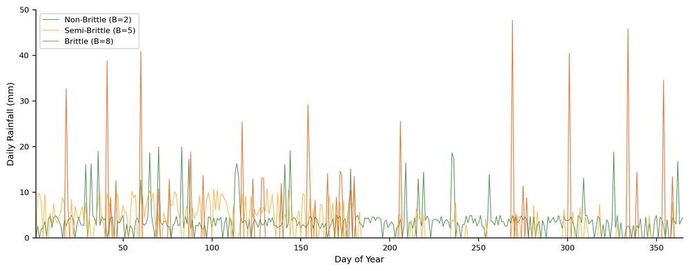
For general illustration, the chart below shows how synthetic daily rainfall patterns differ across brittleness levels. Non-brittle climates (green) have consistent small rainfall events throughout the year. Semi-brittle climates (gold) show distinct wet and dry seasons. Brittle climates (orange) have long dry periods punctuated by intense downpours.
Precip CV (raw) | Brittleness (raw) | Category | Characteristics |
|---|---|---|---|
< 0.30 | 1-2 | Very Non-Brittle | Even rainfall, year-round growth, humid decomposition. |
0.30 to 0.50 | 2-4 | Non-Brittle | Rainfall well spread, short dry season. |
0.50 to 0.70 | 4-6 | Semi-Brittle | Rainfall patchy, longer dry spells. |
0.70 to 1.00 | 6-8 | Brittle | Long dry season; rainfall arrives in bursts. |
≥ 1.0 | 8-10 | Very Brittle | Rainfall erratic; ecosystem inactive for long periods. |
How to read this table alongside the headline score: the table shows the RAW brittleness score derived from CV alone. The score reported in the property profile is the FINAL ecoregion-adjusted score, blending the raw value (70%) with the regional zone baseline (30%). A site whose raw value lands in one band can be reported in an adjacent band once the regional context is applied; the headline category in the property profile is always the final classification.
What this would look like for your land
This Visual Property Atlas is one of four deliverables in the EcoIntel Land Health Report suite. The demonstration property is Wilder Wood Farm; the same analysis applies to any property with at least 1 hectare and 5 years of satellite-observable history.
- Same satellite stack, same scoring engine, same prose.
- Typical turnaround: normally within hours but within 2 working days.
Understand your land by signing up today:
ecointel.io/join • accounts@ecointel.io
Land Health Reports are produced by EcoIntel’s analytical pipeline: 12-platform satellite data integration with AI-synthesised ecological interpretation, calibrated to your property’s regime and ecoregion.